Results

EVAnalyzer stores results in a DuckDB database file named results.evadb inside the project folder:

<image_directory>/evanalyzer/<job_name>/results.evadb

Open an existing results file from the toolbar: click the arrow beside the Open button and select the file.

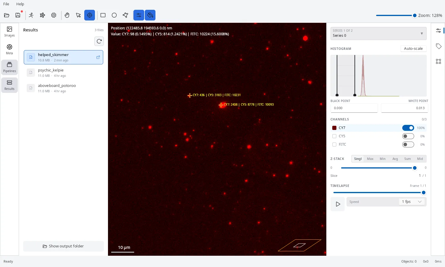
The Results Window

The results window has a left icon rail for switching between the three ways of looking at your data - List, Plate, and Charts - plus an Export shortcut pinned to the bottom. A breadcrumb bar sits above the active view; when your dataset has Z-stacks or time-lapse frames, a Z/T stepper is docked on the right of that same bar and applies to whichever view is currently open.

List View

The List view (the default) shows one row per detected object: Object ID, Image, Class, geometry columns like Area and Circularity, and one Min/Max/Avg/Sum column per measured channel.

The filter bar above the table has three dropdowns - Images, Class, and Columns - each a searchable, multi-select checklist with a X of Y summary (e.g. “19 of 22 Classes”) and select-all/none shortcuts. Columns groups per-channel intensity metrics so you can toggle a whole channel at once instead of column by column. The object count for the current filters is shown at the top-right.

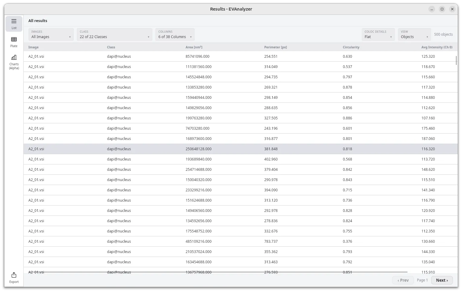
Results are paginated - use ‹ Prev / Next › at the bottom of the table rather than scrolling through everything at once. Click any row to jump straight to that object: EVAnalyzer opens the image it belongs to and highlights it, so you don’t have to hunt for it manually.

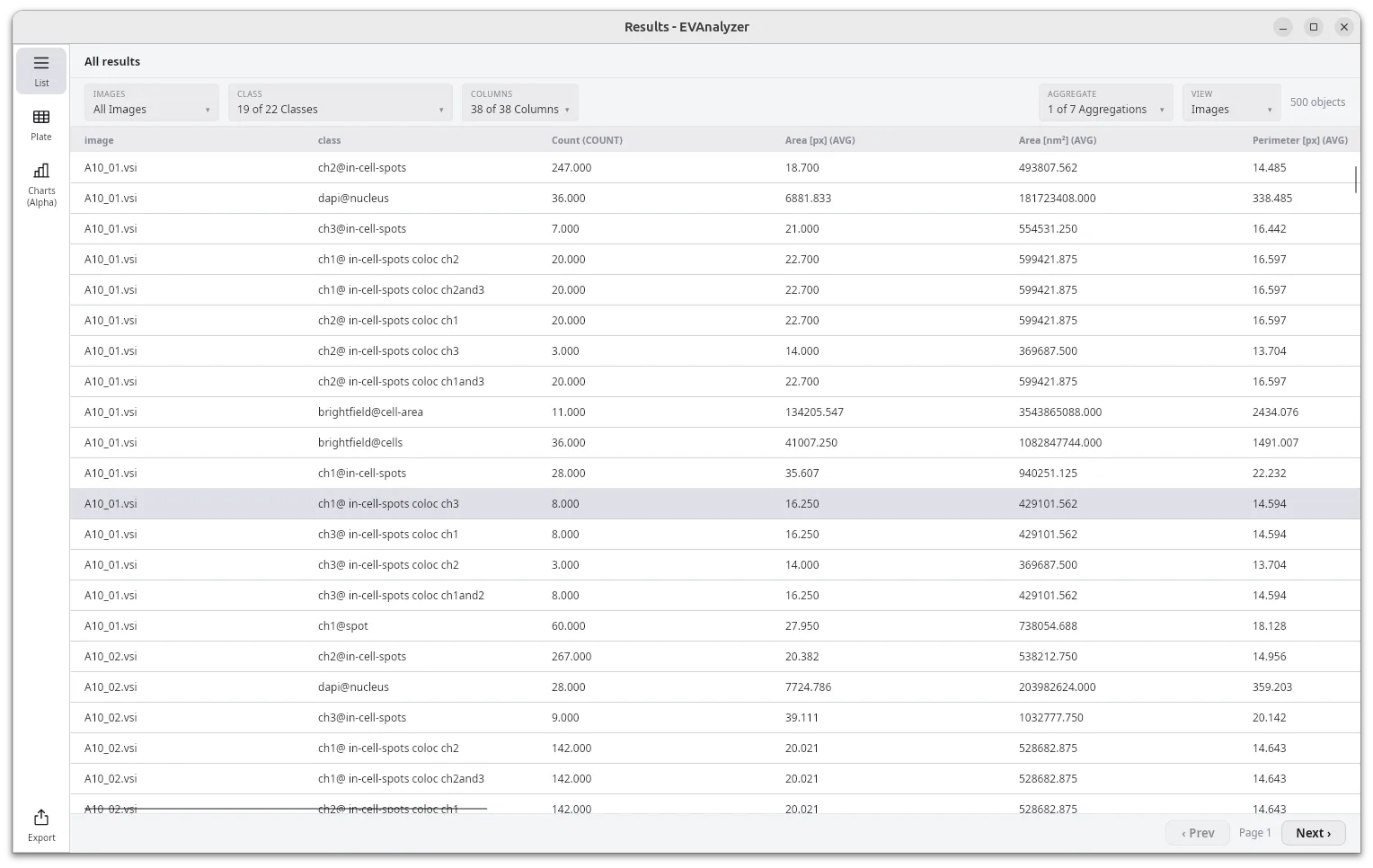
Grouping and Aggregating Rows

Use the View dropdown to switch the table from Objects (flat, one row per object) to Images (one row per image/class combination). Switching to Images reveals an Aggregate dropdown - a multi-select of Average, Min, Max, Std. dev., Sum, Median, and Skewness. Every numeric column is duplicated per selected aggregation (for example Area (px²) [avg] and Area (px²) [sum]), so you can compare, say, average object size against total covered area per image.

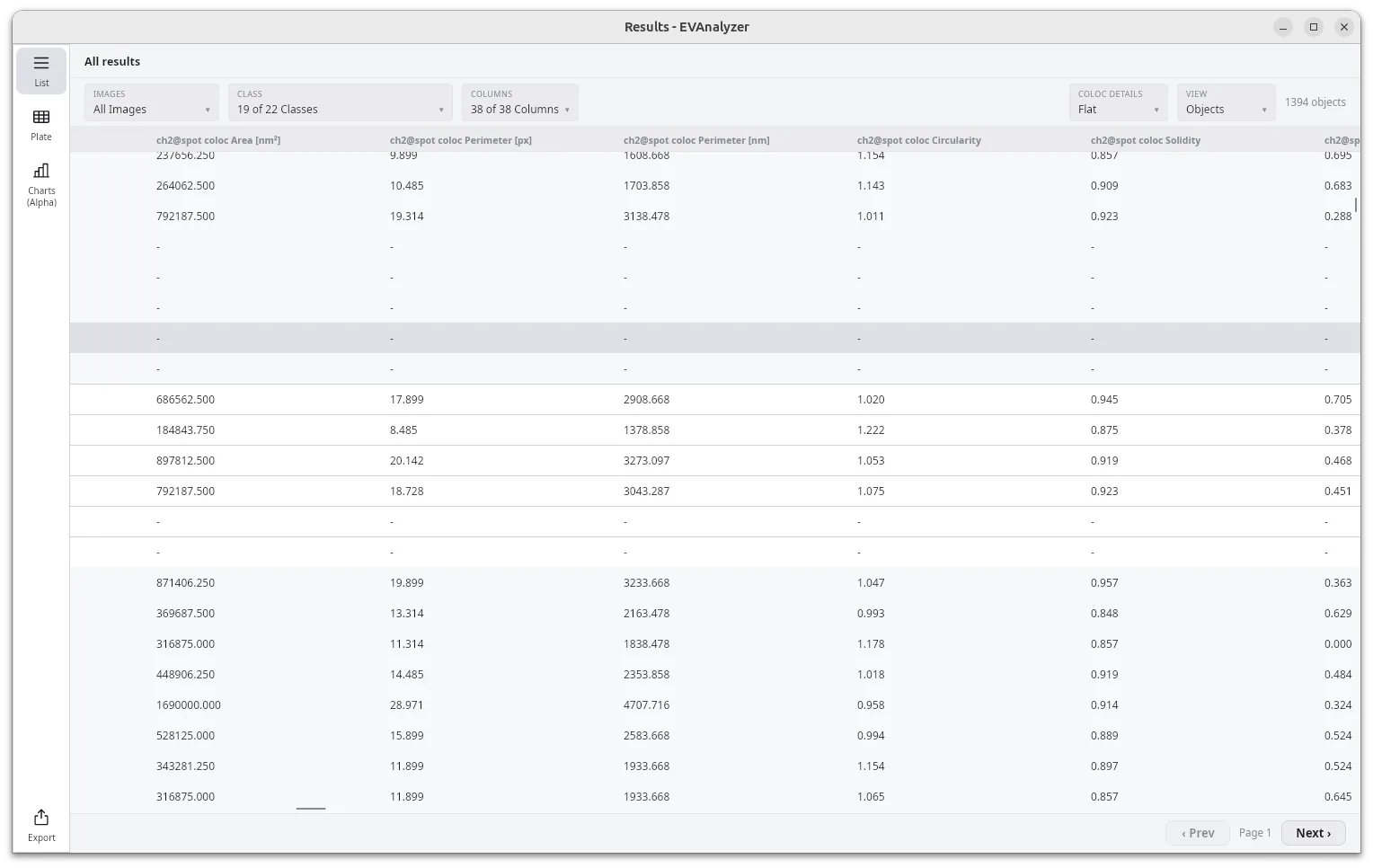
Colocalization Details

While viewing Objects, the Coloc Details dropdown switches between Flat (the default) and Details. Details flattens each object’s matched partners into their own columns - one set of measurement columns per partner class, with a dash where no partner was found.

Charts

The Charts section (marked Alpha in the rail - expect rough edges) plots the currently filtered rows instead of listing them. Three chart types are available as tabs along the top: Histogram, Scatter, and Boxplot.

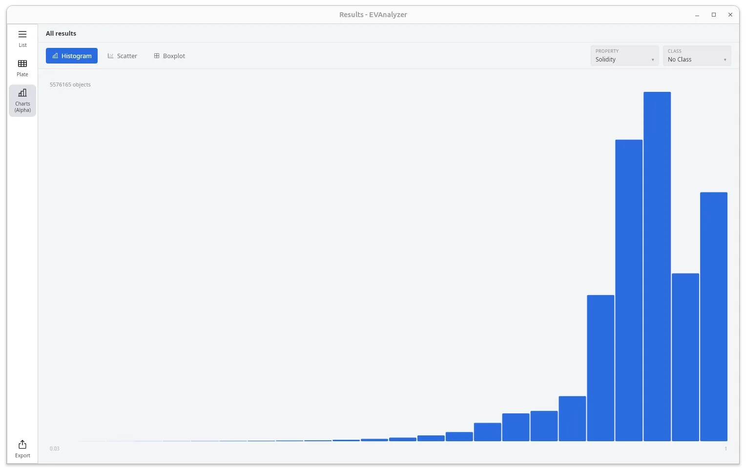
Histogram bins a chosen numeric Property, optionally restricted to one Class, and shows the object count plus the distribution across bins with the value range labelled below.

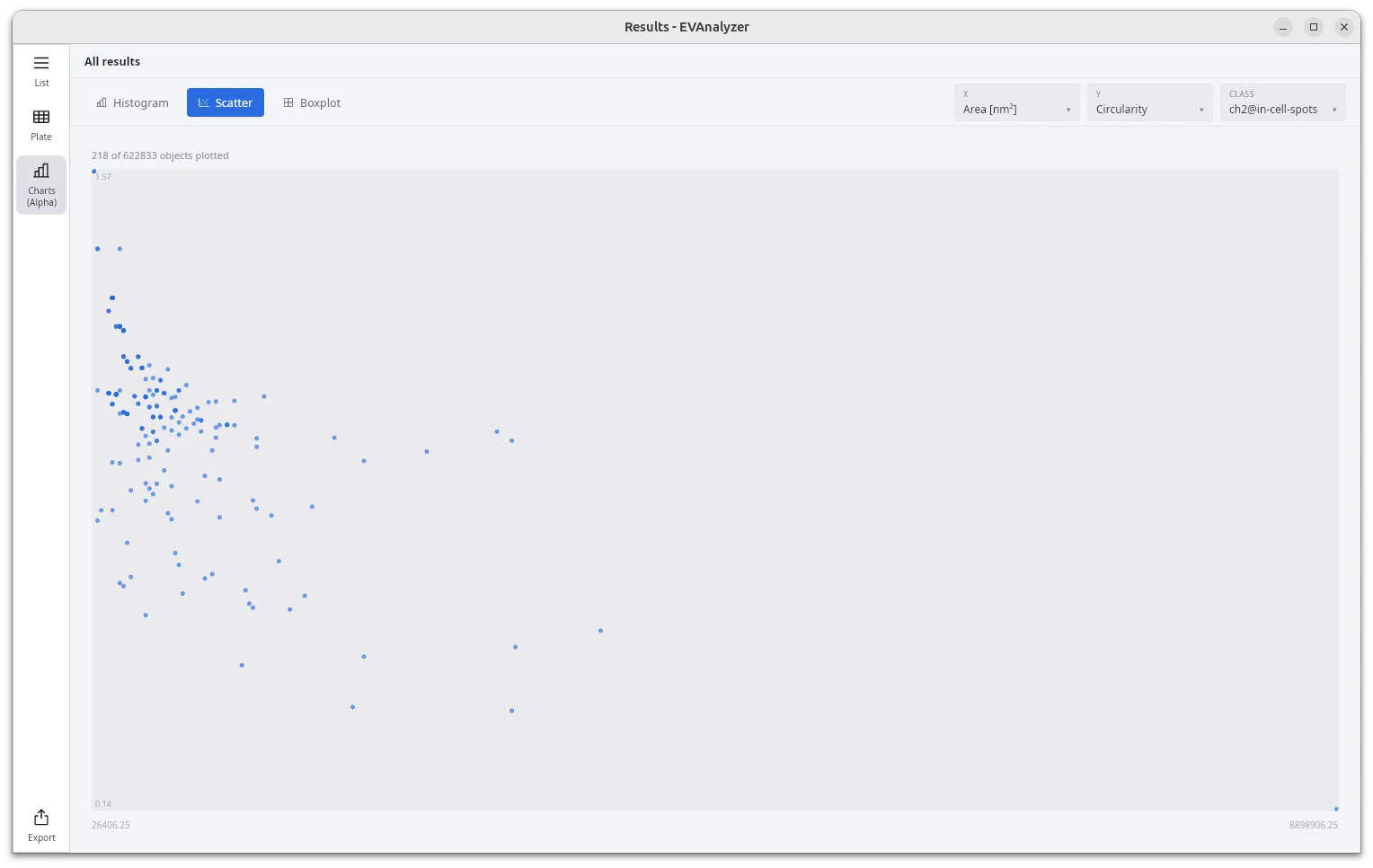
Scatter plots two numeric columns (X and Y), optionally restricted to one Class. Large datasets are downsampled for rendering - a note like “218 of 622833 objects plotted” appears above the plot when this happens.

Boxplot draws one box (quartile box, median line, whiskers, and outlier dots) per class for a chosen Property, with the object count for each class labelled underneath - useful for comparing a metric’s spread across classes at a glance.

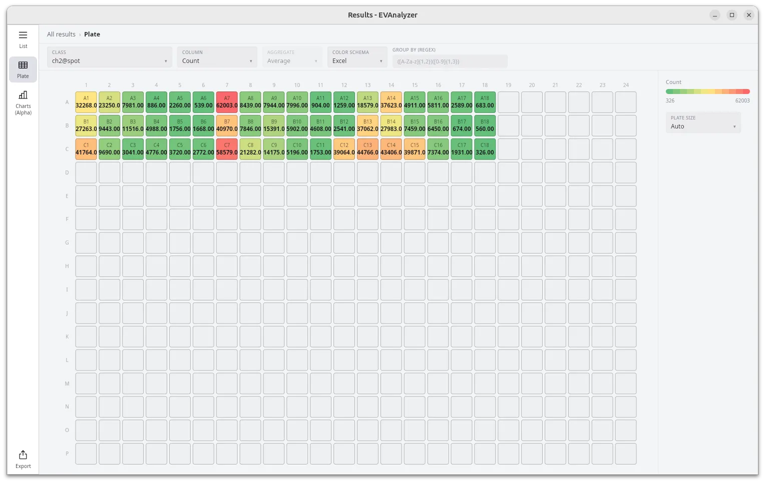
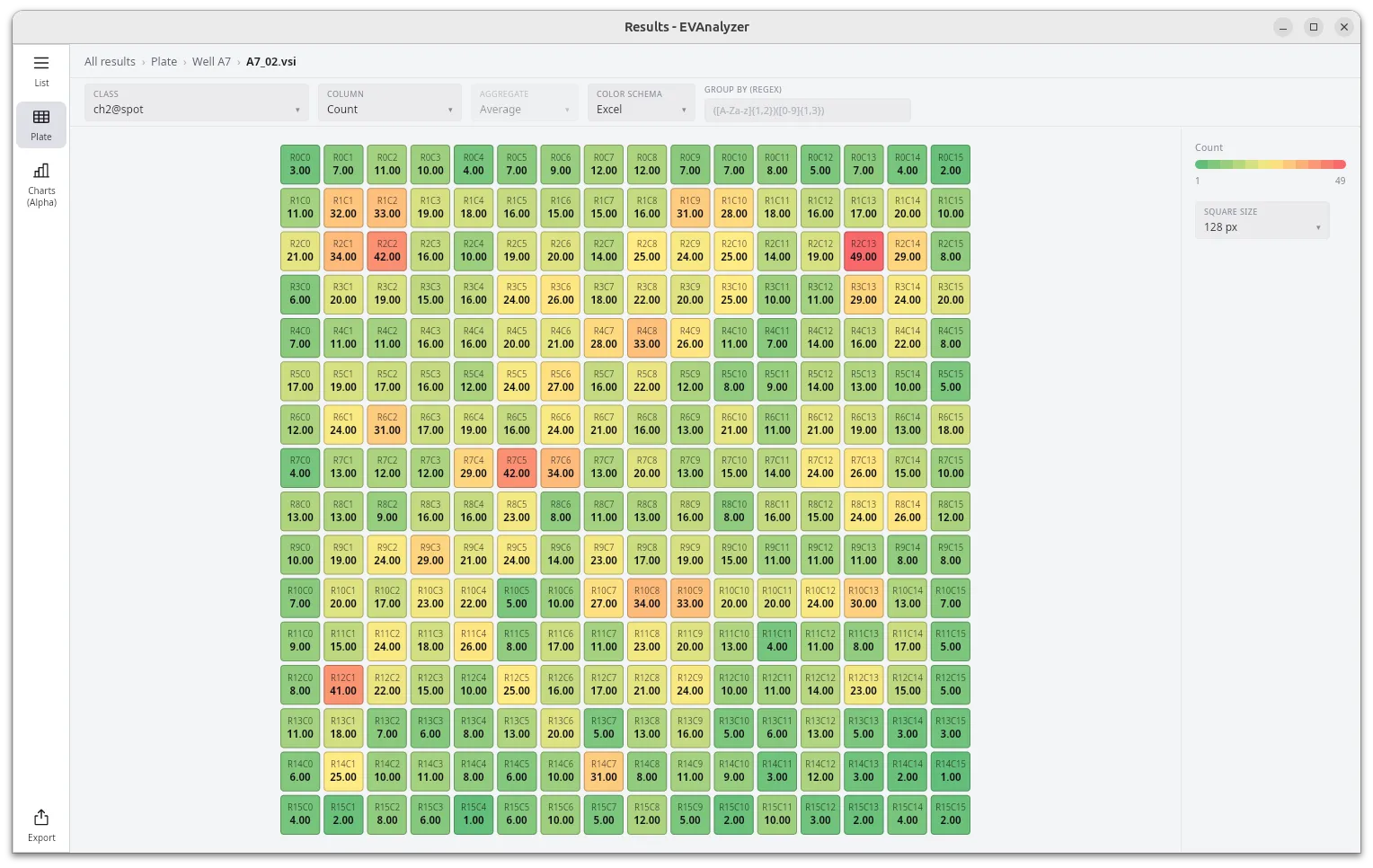
Plate View

Switch to Plate in the rail to lay results out as a physical plate/well grid instead of a table or chart - useful for spotting spatial patterns across a multi-well high-content screening plate. It drills down through three levels, tracked by the breadcrumb at the top: Plate → Well → Image.

A shared toolbar runs across all three levels: Class, Column (the metric to color by), Aggregate, Color Schema (Excel, Viridis, Plasma, Inferno, Cividis, Coolwarm, Red-Blue, YlGnBu, Haline, Algae, or Thermal), and a Group By (regex) field for decoding well/field identifiers out of filenames. A legend on the right shows the active color range - click it to switch between Auto and a Manual min/max.

Plate

Each cell is one well, colored by the aggregated metric across everything grouped into it. Wells are placed by decoding their group label into a row/column coordinate (e.g. A14). Pick a Plate Size - Auto (picks the smallest standard layout that fits your data) or a fixed 6-, 12-, 24-, 48-, 96-, 384-, or 1536-well layout. Click a well to select it and see its value in the side panel, then Open well › to drill in.

Well

Drill into a well to see its individual fields laid out as their own grid (configurable Rows/Cols in the side panel). Click a field to select it, then Open Image › to drill into its spatial heatmap.

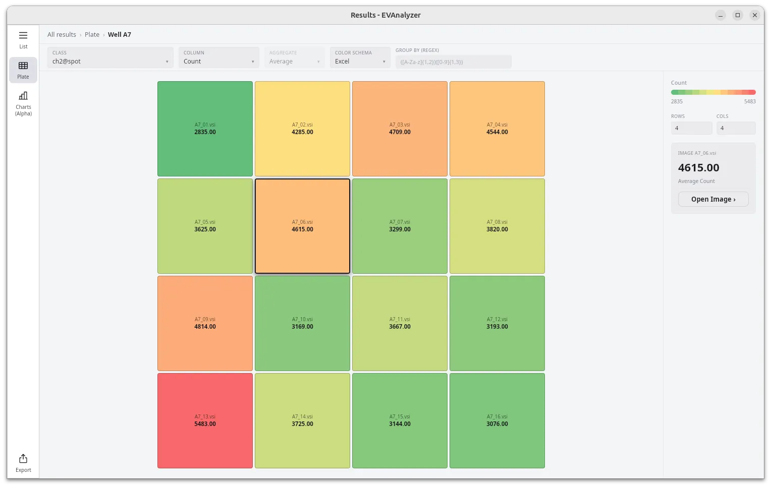
Image Heatmap

The innermost level bins a single image’s objects into square tiles - configure the Square Size (36, 48, 64, 128, 256, or 1024 px) - colored by the same metric/aggregate as the levels above. Click a tile to jump to that region of the image in the editor, highlighted with a rectangle.

Exporting Results

Click Export at the bottom of the rail to open the Export Results dialog. Every checked option is written out together in one run - there’s no separate queue to build up.

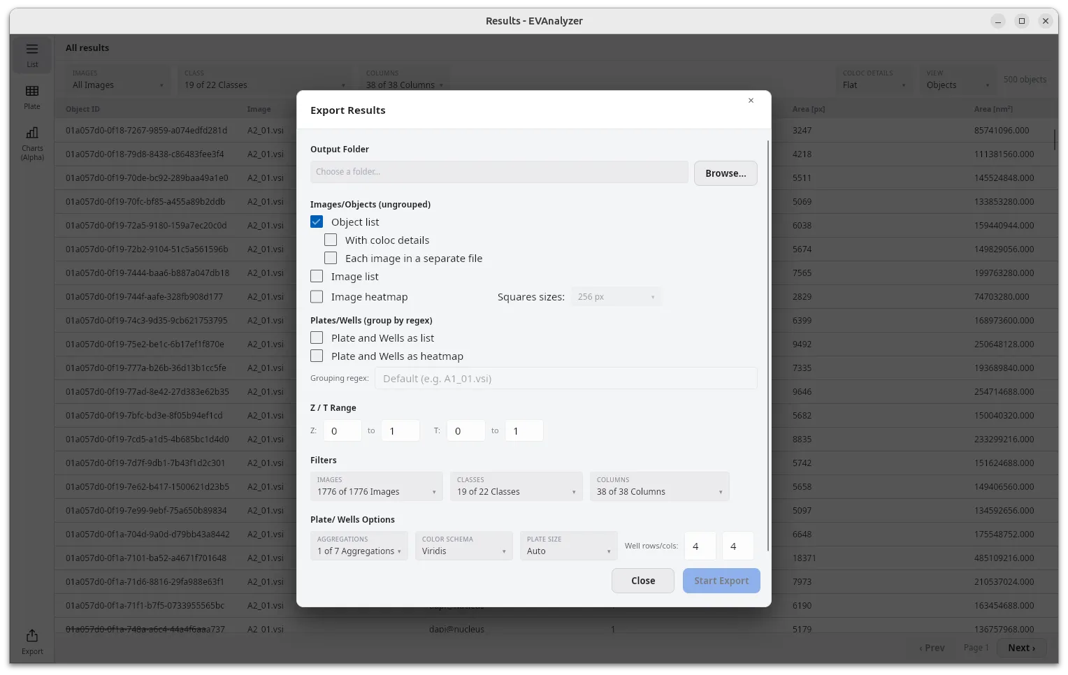
• Output Folder - pick a destination with Browse….
• Format - XLSX (default), CSV, or Parquet.
• Images/Objects (ungrouped) - Object list (with optional With coloc details and Each image in a separate file), Image list (the same aggregated-by-image data as grouping the List view), and Image heatmap (the per-image spatial heatmap grid, with its own Squares sizes setting).
• Plates/Wells (group by regex) - Plate and Wells as list and Plate and Wells as heatmap, both using the Grouping regex field below them (leave it blank to use the default well/field pattern).
• Z/T Range - restrict the export to a Z and/or T plane range.
• Filters - Images, Classes, and Columns, the same multi-select dropdowns as the List view.
• Plate/Wells Options - Aggregations (multi-select), Color Schema, Plate Size, and Well rows/cols, applied to any checked Plate/Well export.

Image heatmap and both Plates/Wells options are XLSX-only - they’re disabled whenever CSV or Parquet is selected. Parquet goes further: picking it ignores every other setting on this page (filters, columns, grouping, checkboxes) and writes a single objects.parquet file - a raw, unfiltered dump of every column in the results database, meant for downstream tools that read Parquet natively rather than for a human to open.

Click Start Export once an output folder is chosen; a progress bar tracks the run and a status message confirms completion or reports an error. For XLSX/CSV, results are named for what they contain (list.xlsx/.csv, grouped_by_image.xlsx/.csv, plate.xlsx, well.xlsx, plate_list.xlsx, well_list.xlsx, heatmap_{image}.xlsx).

Tip

For colocalization exports, partner lookups are resolved in batches of 5,000 source objects at a time - large colocalization datasets export reliably without needing to load everything at once.